 Figure 5.
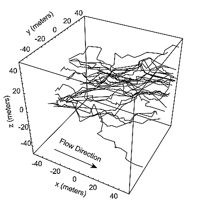
Figure 5. Example transport pathways extracted from a DFN simulation with 20,000 fractures. The pathways were determined by advective particle tracking with mixing at fracture intersections. The examples shown represent only a small fraction of the complete set of 806 pathways. The complete set was used in constructing Figures 6 and 7.
[38] The MARFA code has been used to compute radionuclide decay chain transport in a number of realistic examples that use trajectories extracted from detailed DFN simulations. The example described in this section is based on the DFN simulations described by Cvetkovic et al. [2004]. Those simulations used 20,000 simulated fractures in a 100 m × 100 m × 100 m region and an applied hydraulic gradient of 0.001 m/m. A total of 806 advection-only trajectories representing equally probably pathways were extracted from the flow simulations and input into the MARFA code. The trajectories were generated by releasing particles on the upstream face and tracking those particles advectively through the network. The probability for selecting one of the fractures on the upstream face was proportional to flow in that fracture (flux-weighed release). At each fracture intersection, the advecting particle was assigned randomly to the downstream fractures with probability proportional to the outgoing flux (perfect mixing assumption). The average number of fracture segments per trajectory is about 35. Figure 5 shows 20 of the pathways that were selected randomly from the full set.
[39] The decay chain 241Am → 237Np → 233U → 229Th was used. Mass was released into the pathways as 241Am. The total amount released into all pathways was 1 mole. Note that this is not meant to be a representative release scenario. It is intended purely as a test of the MARFA code to simulate realistic transport scenarios. Two retention models were used: the unlimited diffusion model and the limited diffusion model with an accessible matrix region of 20 mm thickness. Half-lives and retention properties are shown in Table 2. The matrix thickness parameter is used in the limited diffusion model only. The matrix thickness is approximated as infinite in the unlimited diffusion model.
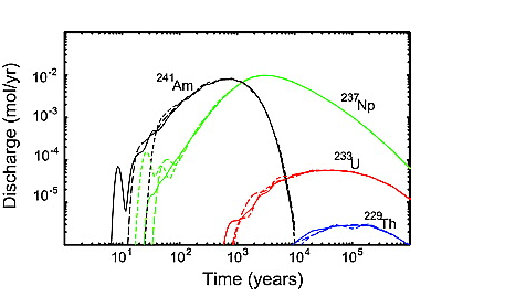 Figure 6.
[40] Results for the infinite diffusion model are shown in Figure 6. For this example, about 76% of the initial mass passes through the 100 m system on a cumulative basis. The remaining mass decayed to one of the decay products of 229Th, which are not tracked. Despite the relatively high cumulative throughput in this example, the mass release is spread over an extremely large time and the amount of mass released in any given year is a small fraction of the released mass (maximum annual discharge is about 10−3 % of the initial pulse). The large spreading in the discharge has two sources. The spreading is caused, in part, by the infinite diffusion model, which has strong kinetic controls. The spreading is also caused by a large variation in traveltime among the different pathways, which is a type of macrodispersion. Note in particular the early arrival time for a small fraction of the mass representing a small number of fast pathways in the DFN.
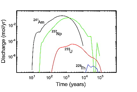 Figure 7.
Figure 7. Discharge versus time for the same scenario as Figure 5, but with the limited diffusion model and a 20 mm accessible matrix region.
[41] Results for the limited diffusion model are shown in Figure 7. Parameters are the same as in Figure 6 except that diffusion is allowed only in a 20 mm matrix region adjacent to the fracture. Peak discharge for the limited diffusion model is about 20 times that of the unlimited diffusion model and occurs at an earlier time. Nearly all of the initial mass passes through the 100 m block with the limited diffusion model.
[42] To appreciate the computational efficiency of the method, note that the particle tracking and reconstruction steps in the large-scale simulations of Figures 6 and 7 took approximately 150 s of computing time for the particle tracking and reconstruction steps. Two broad classes of conventional methods could be used to solve the same problem. In the first conventional approach, a finite element grid would be imposed on each of the 20,000 fractures in the simulation. That approach would require simultaneous solution for a large number of nodal concentrations. The second conventional approach would be to extract the advective trajectories, as in this study, and then solve for concentration on each of the pathways using a conventional numerical code. Although clearly more tractable than full discretization, the second approach would still require 806 individual transport solutions to obtain the ensemble-average breakthrough. Clearly the time domain methods presented here are competitive with these conventional approaches. Part of that computational advantage comes from the fact that the time domain Monte Carlo approach does not need to resolve the transport in each of the 806 pathways. The nature of the Monte Carlo sampling in Figures 6 and 7 is such that the ensemble discharge may be accurately calculated even when the number of particles is too small to accurately resolve the transport in each of the 806 pathways.